# Dr. M. Baron, Statistical Machine Learning class, STAT-427/627

# Polynomial Regression

# Example: QUADRATIC MODEL FOR PREDICTING THE US POPULATION

> setwd("C:\\Users\\baron\\Documents\\Teach\\627 Statistical Machine Learning\\Data")

> Data = read.csv("USpop.csv")

> names(Data)

[1] "Year" "Population"

> attach(Data)

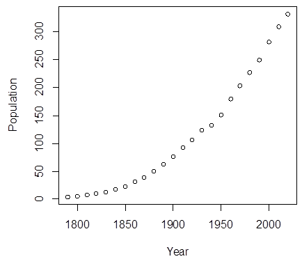
> plot(Year,Population)

# LINEAR MODEL

> lin = lm(Population ~ Year)

> summary(lin)

Call:

lm(formula = Population ~ Year)

Coefficients:

Estimate Std. Error t value Pr(>|t|)

(Intercept) -2.600e+03 1.691e+02 -15.38 2.98e-13 ***

Year 1.425e+00 8.871e-02 16.06 1.24e-13 ***

---

Signif. codes: 0 ‘***’ 0.001 ‘**’ 0.01 ‘*’ 0.05 ‘.’ 0.1 ‘ ’ 1

Residual standard error: 30.08 on 22 degrees of freedom

Multiple R-squared: 0.9214, Adjusted R-squared: 0.9178

F-statistic: 257.9 on 1 and 22 DF, p-value: 1.235e-13

> abline(lin,col="red",lwd=3)

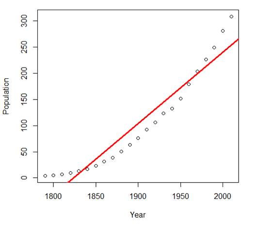
# Clearly, the linear model is too inflexible and restrictive, it does not provide a good fit.

# This is underfitting. Notice, however, that R2 in this regression is 0.9193. Without looking

# at the plot, we could have assumed that the model is very good!

> predict(lin,data.frame(Year=2030))

1

291.5174

# This is obviously a poor prediction. The US population was already 331 million during the most

# recent Census. So, we probably omitted an important predictor. Residual plots will help us

# determine which one.

# Let’s produce various related plots. Partition the graphics window into 4 parts and use “plot”.

> par(mfrow=c(2,2))

> plot(lin)

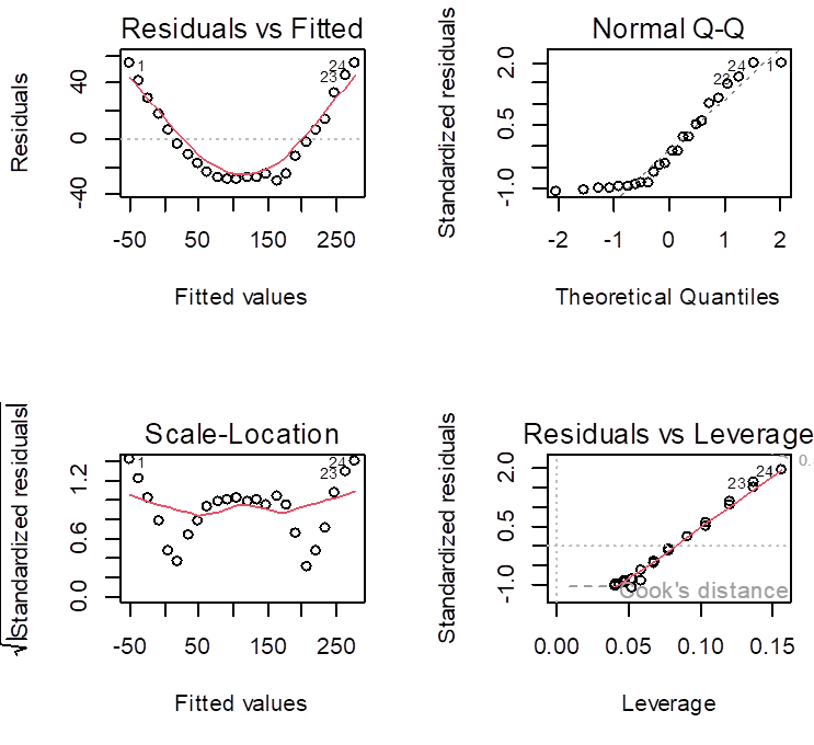
# The first plot shows that a quadratic term has been omitted although

# it is important in the population growth. So, fit a quadratic model.

# Command I(…) means “inhibit interpretation”, it forces R to understand (…)

# literally, as Year squared.

> quadr = lm(Population ~ Year + I(Year^2))

> summary(quadr)

Estimate Std. Error t value Pr(>|t|)

(Intercept) 2.170e+04 5.227e+02 41.52 <2e-16 ***

Year -2.412e+01 5.493e-01 -43.91 <2e-16 ***

I(Year^2) 6.705e-03 1.442e-04 46.51 <2e-16 ***

---

Signif. codes: 0 ‘***’ 0.001 ‘**’ 0.01 ‘*’ 0.05 ‘.’ 0.1 ‘ ’ 1

Residual standard error: 3.019 on 21 degrees of freedom

Multiple R-squared: 0.9992, Adjusted R-squared: 0.9992

F-statistic: 1.389e+04 on 2 and 21 DF, p-value: < 2.2e-16

# A higher R-squared is not surprising. It will always increase when we add

# new variables to the model. The fair criterion is Adjusted R-squared, when

# we compare models with a different number of parameters. Quadratic model has

# Adjusted R-squared = 0.999 comparing with 0.9155 for the linear model.

# Now let’s obtain the fitted values and plot the fitted curve.

> Yhat = fitted.values(quadr)

> lines(Year,Yhat,col="blue",lwd=3)

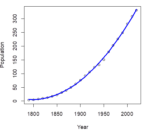
# The quadratic curve fits nearly perfectly. The quadratic growth slowed down only during

# the World War II, although Baby Boomers quickly caught up with the trend.

> predict(quadr,data.frame(Year=2030))

1

364.1572

# Now, this is a reasonable prediction for the year 2030.

> predict(quadr,data.frame(Year=2030),interval="confidence")

fit lwr upr

1 364.1572 359.9686 368.3459

> predict(quadr,data.frame(Year=2030),interval="prediction")

fit lwr upr

1 364.1572 356.6102 371.7042

# Food for thought... Are the confidence and predictions intervals valid here?